Hybrid Generative-Discriminative Deep Models
Deep discriminative classifiers perform remarkably well on problems with a lot of labeled data. So-called deep generative models tend to excel when labeled training data is scarce. Can we do a hybrid, combining the best of both worlds? In this post I outline a hybrid generative-discriminative deep model loosely based on the importance weighted autoencoder (Burda et al., 2015). Don’t miss the pretty pictures.
Discriminative vs Generative Classifiers
Ok, let’s say we have a dataset $\set{ \vect{x_i}, y_i }, i = 0 … N$ and we want to train a classifier that can infer a label $y_i$ from an example $\vect{x_i}$. There are essentially two different ways to go about that:
-
you train a model to approximate $p(y \given \vect{x})$ directly, or
-
you train a model to approximate $p(\vect{x}, y)$, and then use the definition of conditional probability to compute $p(y \given \vect{x})$ as $p(\vect{x}, y) / p(\vect{x})$.
In the first case the resulting classifier is called a discriminative classifier; in the second case it’s called a generative classifier. Each has its strengths and weaknesses: A generative classifier typically does better when there is little labeled training data ($N$ is relatively small), while a discriminative one does better on larger datasets, or at least asymptotically as $N \rightarrow \infty$ (Ng et al., 2001).
Another common weakness of generative models is that they often require that the model be evaluated once for every possible label $y$, i.e. to do inference we compute $p(\vect{x}, y)$ for every possible $y$ and choose the label with the highest probability. A discriminative model, in contrast, typically computes the probability of every label in one pass. This of course is a major advantage on classification problems with many (perhaps thousands of) labels.
So how can we combine the strengths of both approaches in one model, while avoiding the weaknesses?
Generative vs Discriminative Assumptions
In generative models we usually assume that a latent variable $\vect{z}$ was somehow involved in the generation of our dataset. The typical genesis narrative thus goes something like this:
-
first the latent variable $\vect{z}$ was sampled from some prior distribution $p(\vect{z})$,
-
then the data point $\vect{x}$ was drawn from the conditional distribution $p(\vect{x} \given \vect{z})$, and
-
finally the label $y$ was drawn from the conditional distribution $p(y \given \vect{z}, \vect{x})$;
meaning we can write the full joint probability function as:
$$ \begin{equation} p(\vect{x}, \vect{z}, y) = p(\vect{z}) p(\vect{x} \given \vect{z}) p(y \given \vect{x}, \vect{z}) \end{equation} $$
The latent variable $\vect{z}$ is typically considered a nuisance parameter and we (attempt to) integrate it out:
$$ \begin{equation} p(\vect{x}, y) = \int p(\vect{z}) p(\vect{x} \given \vect{z}) p(y \given \vect{z}, \vect{x}) dz \end{equation} $$
Now let’s take a closer look at $p(y \given \vect{z}, \vect{x})$: if we make the simplifying Markov assumption that $y$ is conditionally independent of $\vect{z}$ given $\vect{x}$, i.e. that all the information needed to generate $y$ is available in $\vect{x}$, then we can approximate it as $q(y \given \vect{x}).$ Eq. 2 then becomes
$$ \begin{equation} p(\vect{x}, y) \approx \int p(\vect{z}) p(\vect{x} \given \vect{z}) q(y \given \vect{x}) dz. \end{equation} $$
Since $q(y \given \vect{x})$ is independent of $\vect{z}$ we can bring it out of the integral
$$ \begin{equation} p(\vect{x}, y) \approx q(y \given \vect{x}) \int p(\vect{z}) p(\vect{x} \given \vect{z}) dz, \end{equation} $$
and what remains inside the integral is just $p(\vect{x})$. So Eq. 4 essentially just says $p(\vect{x}, y) \approx q(y \given \vect{x}) p(\vect{x})$, which is the same as $p(y \given \vect{x}) \approx q(y \given \vect{x})$. This is the quintessential discriminative model. So it seems that, from a generative perspective, the fundamental assumption behind a discriminative classifier is the simplifying Markov assumption that $p(y \given \vect{z}, \vect{x}) \approx q(y \given \vect{x})$.
Now let’s see what happens if we make the alternative simplifying Markov assumption and assume that $p(y \given \vect{z}, \vect{x}) \approx q(y \given \vect{z})$, i.e. that the latent variable $\vect{z}$ contains all the information necessary to generate the label $y$. Then
$$ \begin{equation} p(\vect{x}, y) \approx \int p(\vect{z}) p(\vect{x} \given \vect{z}) q(y \given \vect{z}) dz. \end{equation} $$
If you’re familiar with the litterature on variational autoencoders (Kingma et al., 2014; Rezende et al., 2014) then this should be recognizable as a generative model (for the joint $\vect{x’} = \set{\vect{x}, y}$) that fits nicely into that framework.
So what happens if we attempt to make a trade-off between those two simplifying assumptions?
A Hybrid Generative-Discriminative Deep Model
Let’s say we assume that $p(y \given \vect{z}, \vect{x})$ can be approximated by a linear combination (mixture) of a $q(y \given \vect{x})$ and a $q(y \given \vect{z})$. Eq. 2 then becomes
$$ \begin{equation} p(\vect{x}, y) \approx \int p(\vect{z}) p(\vect{x} \given \vect{z}) (\beta q(y \given \vect{x}) + (1 - \beta) q(y \given \vect{z})) dz. \end{equation} $$
Note that for $\beta = 1$ this is a purely discriminative model, and for $\beta = 0$ a generative one. Hopefully, somewhere in between there’s a good trade-off for each given problem.
So how do we transform Eq. 6 into something we can attack with stochastic gradient descent?
Parameterization and optimization
We start by noting that the integral in Eq. 6 can be Monte Carlo approximated with importance sampling, along lines similar to those drawn up by Burda et al. (2015). We start by introducing $q(\vect{z} \given \vect{x})$ as the distribution we will importance sample from, and $q(\vect{x} \given \vect{z})$ as an approximation to $p(\vect{x} \given \vect{z})$. With $q(y \given \vect{z}, \vect{x}) = \beta q(y \given \vect{x}) + (1 - \beta) q(y \given \vect{z})$ we then get
$$ \begin{equation} p(\vect{x}, y) \approx \int q(\vect{z} \given \vect{x}) \frac{p(\vect{z})}{q(\vect{z} \given \vect{x})} q(\vect{x} \given \vect{z}) q(y \given \vect{x}, \vect{z}) dz. \end{equation} $$
This can be seen as an expectation over $q(\vect{z} \given \vect{x})$ and we can thus approximate it with a finite number of samples as
$$ \begin{equation} p(\vect{x}, y) \approx \frac{1}{K} \sum_{i=0}^{K} \left[ \frac{p(\vect{z})}{q(\vect{z} \given \vect{x})} q(\vect{x} \given \vect{z}) q(y \given \vect{x}, \vect{z}) \right]_{\vect{z} \sim q(\vect{z} \given \vect{x})} \end{equation} $$
Now we simply choose distribution families for $q(\vect{z} \given \vect{x})$, $q(\vect{x} \given \vect{z})$, $q(y \given \vect{x})$ and $q(y \given \vect{z})$ and parameterize them as deep neural networks. Exactly which distribution families to choose and how to structure the deep neural networks depends on the problem at hand, but it should be noted that composition of the neural networks representing $q(\vect{z} \given \vect{x})$ and $q(y \given \vect{z})$ essentially gives a neural network representation of $q(y \given \vect{x})$. This is an opportunity for weight sharing at the very least.
It can also be noted that $y$ need not appear as input anywhere.
The neural networks representing
$q(y \given \vect{z}, \vect{x})$ can thus output a categorical distribution through a
softmax layer. This lets the model scale to problems with a large number of
labels.
Experiments
I’ve implemented the model described above in this Jupyter notebook and trained it on a toy dataset. For this rudimentary implementation I used fully connected neural networks two layers deep, and a two-dimensional factorized normal distribution for the latent space $\vect{z}$. You can see the result below.
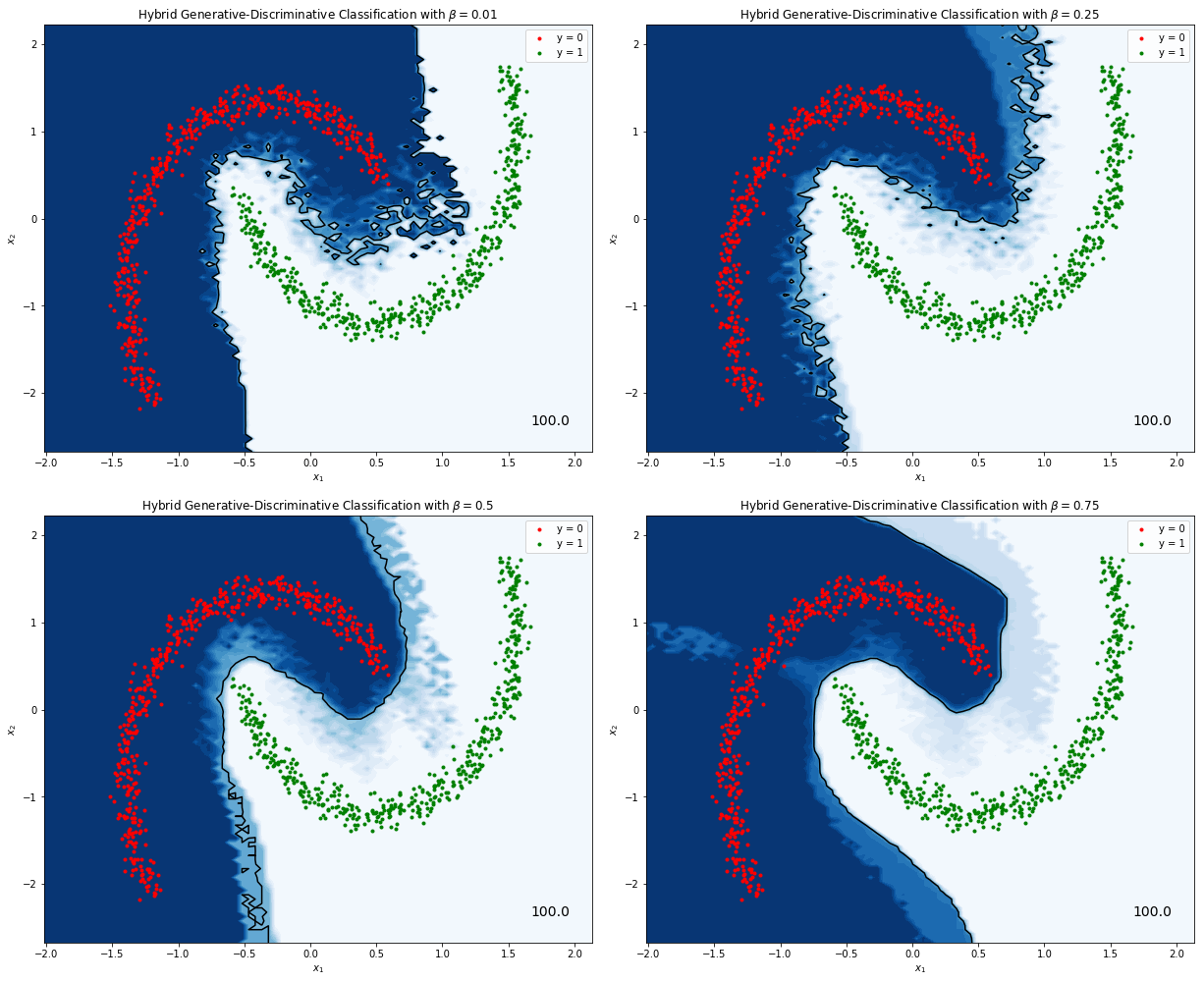
Figure 1. Hybrid generative-discriminative classifiers trained on a toy dataset. In the top left corner a predominantly generative classifier ($\beta = 0.01$), and then progressively more discriminative ones ($\beta = 0.25$, $\beta = 0.5$ and $\beta = 0.75$).
Next Steps
I’m not sure how novel this approach is or how well it will perform on real datasets. I just thought I’d throw the idea out there and see if it sticks. If you see a good use case or want to explore this idea further please don’t hesitate to contact me.
Given that results on real datasets warrant further work there’s one rather obvious possible improvement: A lot of progress has been done lately on expressive latent distributions. It would be interesting to see this approach combined with e.g. real-valued non-volume preserving transformations (Dinh et al., 2016) or inverse autoregressive flow (Kingma et al., 2016).
Don’t hesitate to shoot me an email or ping me on Twitter if you’re interested in working on this!